Aggregate expenditure and equilibrium output. Aggregate Expenditure and Equilibrium Output Flashcards 2023-01-04

Aggregate expenditure and equilibrium output Rating: 8,2/10 1445 reviews

Aggregate expenditure is the total amount of money that households, firms, and the government spend on goods and services in an economy. This includes consumer spending, investment spending by firms, and government spending. Equilibrium output, also known as full employment output or potential output, is the level of output produced by an economy when all of its resources are being used efficiently and there is no excess capacity.

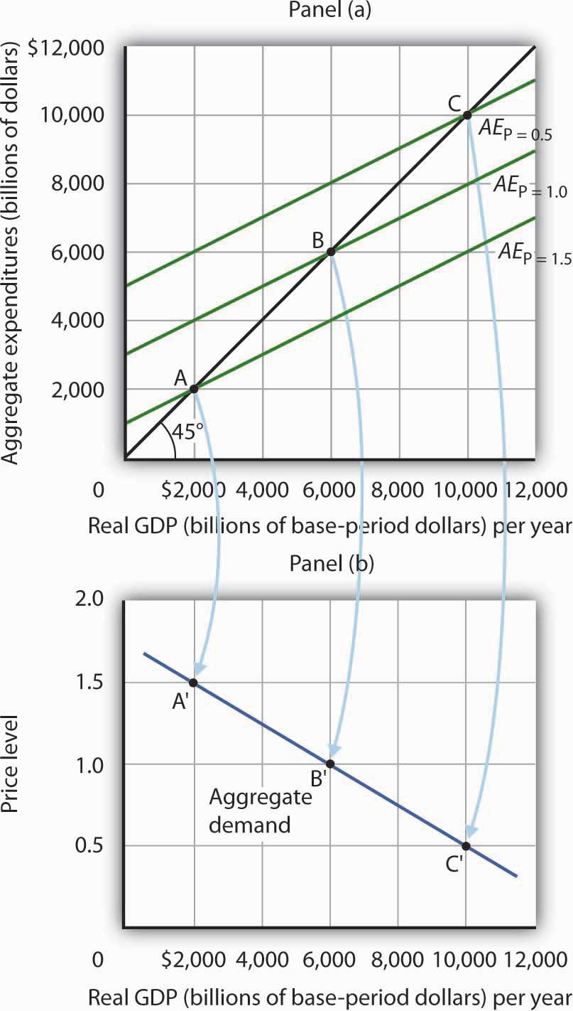
In economics, the relationship between aggregate expenditure and equilibrium output is analyzed using the aggregate demand (AD) curve. The AD curve shows the relationship between the price level of goods and services and the quantity of goods and services demanded by households, firms, and the government. As the price level increases, the quantity of goods and services demanded decreases, and vice versa.

The intersection of the AD curve and the aggregate supply (AS) curve determines the equilibrium output of an economy. The AS curve shows the relationship between the price level and the quantity of goods and services that firms are willing and able to produce. When the AD curve intersects the AS curve at a point above the full employment output level, there is excess demand for goods and services, which leads to an increase in the price level and an increase in output. Conversely, when the AD curve intersects the AS curve at a point below the full employment output level, there is excess supply of goods and services, which leads to a decrease in the price level and a decrease in output.

There are several factors that can shift the AD curve. An increase in government spending, for example, will shift the AD curve to the right, resulting in a higher equilibrium output. Similarly, an increase in the level of household income will also shift the AD curve to the right, as households will have more money to spend on goods and services. On the other hand, a decrease in the level of household income will shift the AD curve to the left, resulting in a lower equilibrium output.

It is important to note that while changes in aggregate expenditure can affect the level of equilibrium output, they do not necessarily affect the unemployment rate. The unemployment rate reflects the percentage of the labor force that is not employed but is actively seeking work. An increase in aggregate expenditure may lead to an increase in output and employment, but it could also lead to an increase in the labor force as more people enter the job market.

In conclusion, aggregate expenditure and equilibrium output are closely related concepts in economics. Aggregate expenditure represents the total amount of money spent on goods and services in an economy, while equilibrium output is the level of output produced when all resources are being used efficiently. The AD curve shows the relationship between aggregate expenditure and the price level of goods and services, while the AS curve shows the relationship between the price level and the quantity of goods and services that firms are willing and able to produce. Changes in aggregate expenditure can affect the level of equilibrium output, but they do not necessarily affect the unemployment rate.

28.2 The Aggregate Expenditures Model

aggregate expenditure and equilibrium output

Coffee and donut shops have coffee and snacks available to customers when they walk in. Planned changes in inventories are already included in planned investment and aggregate expenditure. In Chapter 5 and at the beginning of this chapter, we used an aggregate demand and aggregate supply model to explain business cycle fluctuations in real GDP and employment. The marginal propensities to consume and import describe the changes in aggregate expenditure caused by changes in income. We can use the aggregate expenditures model to gain greater insight into the aggregate demand curve. The line has a slope equal to one.


Next

6.5 Equilibrium output and the AD curve

aggregate expenditure and equilibrium output

ΔI MPC ΔI MPC ΔI MPC ΔI. For example, assume as shown in the diagram, that output and incomes are only Y 1. The multiplier effect works because a change in autonomous aggregate expenditures causes a change in real GDP and disposable personal income, inducing a further change in the level of aggregate expenditures, which creates still more GDP and thus an even higher level of aggregate expenditures. . As we will see in later chapters, the tax cut helped push the economy into a period of rising inflation. As part of the analysis, in the article he mentioned that he assumed an MPC of about two-thirds, since many households at the time were living paycheck-to-paycheck. In short-run equilibrium, output equals the total of goods and services households, businesses, and residents of other countries want to buy.

Next

6.3: Aggregate expenditure and equilibrium output in the short run

aggregate expenditure and equilibrium output

In general, any change in autonomous aggregate expenditures shifts the aggregate demand curve. . Occurs when there is no tendency for change. If aggregate expenditures equal real GDP, then firms will leave their output unchanged; we have achieved equilibrium in the aggregate expenditures model. The size of the horizontal shift would be. And there will be less than planned inventory when sales are stronger than expected.

Next

Macroeconomics Chapter 8: Aggregate Expenditure and Equilibrium Output Flashcards

aggregate expenditure and equilibrium output

The relationship between consumption and income. D either increase or decrease depending on the size of the change in investment. Since E is the only point on the AE line also on the line, it is the only point at which output and planned expenditure are equal. In this chapter we have developed a basic explanation for the shifts in AD that cause changes in real output. Either response—unplanned inventory reductions or turning away customers—is a signal to firms that aggregate expenditure is greater than current output, markets are strong, and output and sales can be increased profitably. An increase in the price level would reduce the real value of this money, reduce your real wealth, and thus reduce your consumption. The Aggregate Expenditures Model: A Simplified View To develop a simple model, we assume that there are only two components of aggregate expenditures: consumption and investment.

Next

Aggregate_Expenditure_and_Equilibrium_Output (1).doc

aggregate expenditure and equilibrium output

A lower price level will increase exports and reduce imports, increasing net exports. The lower the price level, the higher the aggregate expenditures curve and the higher the equilibrium level of real GDP. The Aggregate Expenditures Model in a More Realistic Economy Four conclusions emerge from our application of the aggregate expenditures model to the simplified economy presented so far. We turn now to an investigation of the relationship between the marginal propensity to consume and the multiplier. The consumption function relates the level of consumption in a period to the level of disposable personal income in that period. Aggregate expenditure and equilibrium output in the short run 135 In Figure6. The economy had slipped into a recession in 1960.

Next

Aggregate Expenditure and Equilibrium Output Flashcards

aggregate expenditure and equilibrium output

As before, we assume that the marginal propensity to consume is 0. He reasoned that making various tax cuts permanent would have little impact on consumption now, since households in 2008 were cash-strapped. Household wealth: higher wealth leads to higher spending and saving. If autonomous expenditure increased from A 0 to A 1 as shown in panel a , equilibrium output would increase from Y 0 to. The process continues, thus multiplying the impact of the reduction in aggregate expenditures resulting from the reduction in planned investment. Income Y 2 is the only income at which aggregate expenditure just buys all current output. This added purchasing power would generate still further increases in spending and incomes.

Next

Aggregate expenditure and equilibrium output in the short run

aggregate expenditure and equilibrium output

. D income in the economy will fall because the decreased consumption that results from increased saving causes the economy to contract. It is the amount of aggregate expenditures C + I P + G + X n when real GDP is zero. An aggregate consumption function shows that the upward slope indicates that higher levels of income lead to higher levels of consumption spending. The level of consumption at the intersection of the consumption function and the vertical axis is regarded as autonomous consumption; this level of spending would occur regardless of the level of real GDP.

Next

28.3 Aggregate Expenditures and Aggregate Demand

aggregate expenditure and equilibrium output

We get the following: Equation 28. But, as president he proposed the tax cut in 1962. The former do not vary with GDP; the latter do. In this section we shall see how to derive the aggregate demand curve from the aggregate expenditures model. The intercept of the aggregate expenditures curve shows the level of autonomous aggregate expenditures.

Next

Chapter 8 Aggregate Expenditure and Equilibrium Output 2f0cb1f8d442732650 f356949 d1466f8

aggregate expenditure and equilibrium output

For example, assume as shown in the diagram, that output and incomes are only Y 1. The equations for the simplified economy are easier to work with, and we can readily apply the conclusions reached from analyzing a simplified economy to draw conclusions about a more realistic one. What is its slope? As a result, if planned expenditure AE and GDP are different then plans in some part of the economy have not been realized and there is an incentive to change output. There will be more than planned inventory when sales are overestimated. Notice first that the intercept of the AE curve in Panel b is higher than that of the AE curve in Panel a.

Next