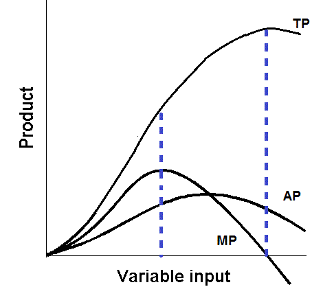
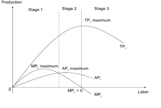
The marginal product curve is a graphical representation of the relationship between the marginal product of a variable input and the level of that input. The marginal product of an input is the additional output that is generated as a result of using one more unit of that input, holding all other inputs constant.
For example, consider a firm that produces widgets using two inputs: labor and capital. The marginal product of labor is the additional output that is generated as a result of hiring one more worker, holding the level of capital constant. Similarly, the marginal product of capital is the additional output that is generated as a result of using one more unit of capital, holding the level of labor constant.
The marginal product curve for a particular input shows the relationship between the marginal product of that input and the level of that input. The curve typically starts at a high point and then decreases as the level of the input increases. This is because the marginal product of an input tends to decline as more of that input is used.
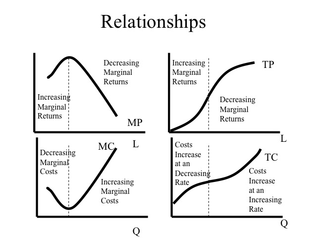
There are several reasons why the marginal product curve might decline. One reason is the law of diminishing returns, which states that as more of a particular input is used, the marginal product of that input will eventually decline. This is because there are only a certain number of ways that the input can be used effectively, and at some point the marginal product will begin to decrease as the input is used in less and less efficient ways.
Another reason why the marginal product curve might decline is because of the presence of fixed inputs. Fixed inputs are inputs that cannot be varied in the short run, such as the factory in which a firm produces its goods. If the level of a fixed input is not sufficient to support the level of production desired, then the marginal product of variable inputs will decline as those inputs are used in increasingly inefficient ways.
The marginal product curve is an important concept in economics because it helps to explain the behavior of firms and the allocation of resources. By understanding the marginal product curve, firms can make more informed decisions about how to allocate their inputs in order to maximize output and profits. It is also a key concept in the analysis of supply and demand, as it helps to explain how firms respond to changes in the price of inputs.
In conclusion, the marginal product curve is a graphical representation of the relationship between the marginal product of a variable input and the level of that input. It is an important concept in economics that helps to explain the behavior of firms and the allocation of resources, and it plays a key role in the analysis of supply and demand.
Chapter 11 micro Flashcards

This usually translates to a diminishing level of profitability per car. A Technology involves research and development while technological change involves the use of more efficient machinery. So, the total change in output produced by the company comes to 50,000 units 150,000 — 100,000. In the case of the federal government, it refers to the total amount of income generated from taxes, which remains unfiltered from any deductions. Currently, the average product of labor is 120 pounds of avocados per day. In this case, the vertical change is q minus zero, since the line starts at the origin, and the horizontal change is L minus zero.
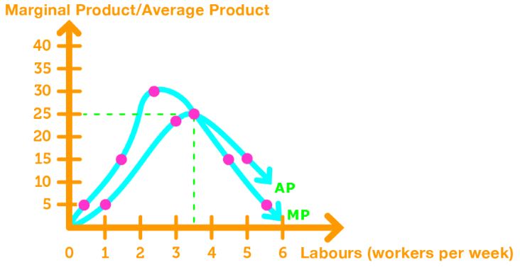
Relationship between Marginal Product and Average Product

B As output increases, average fixed cost becomes smaller and smaller. For example, if adding another worker increases output by more than the average product of the total labor force, then the marginal product of the new worker will raise the average product amount. A Toyota builds a new assembly plant in Texas. Then, divide the same by the difference in the factor of production. Calculate Vipsana's average fixed cost per day when she produces 50 gyros using two workers? Graphically, the two are illustrated as mirror images to one another. D additional cost of producing an additional unit of output. Which of the following statements correctly describes the distinction between technology and technological change? Step 2: Next, determine the final production output and the corresponding labor input which are denoted by Y 1 and L 1 respectively.
Marginal and Average Product Curves (With Diagram)

As a result, he reduced the number of factor units to equal the price of each factor unit. B Diminishing returns are the result of changes in explicit costs. B Marginal cost will equal average total cost when marginal cost is at its lowest point. We quantify the units of labour along with the horizontal axis and the output end result along with the vertical axis. You are free to use this image on your website, templates, etc. Still, there will be a certain point where there will be no increase in the output, and they will also start falling, or the same may even become negative. They replace the expensive factors with cheaper ones.
Marginal Productivity

But, in the later stage, it gives declining returns due to a massive increase in factor units. D When marginal cost is greater than average fixed cost, average fixed cost increases. At this point, the entrepreneur reduces the number of factor units to OQ1. Inputs include land, labor, capital, technology, and entrepreneurship. B additional output when total cost is increased by one dollar. In contrast, as the price of the factor increases to OP1, the additional productivity is the highest i.
