Short run marginal cost formula. Production In The Short Run 2022-12-21
Short run marginal cost formula Rating:
8,3/10
570
reviews
The poem "Two Tiny Feet" is a poignant and emotional tribute to the life of a newborn child. The poem speaks to the joy and wonder that comes with the arrival of a new baby, as well as the deep love and commitment that parents feel for their child.
The poem begins by describing the "two tiny feet" of the newborn, which are described as being "so perfect and so small." These feet represent the innocence and vulnerability of the child, as well as the endless potential that lies within them. The poet goes on to describe the child's "little hands" and "tiny fingers," which are also described as being delicate and perfect.
The poem then shifts to focus on the feelings of the parents, as they gaze upon their new child with love and wonder. The poet writes of how the parents "look with love upon this precious child," and how they are filled with "hope and joy" at the prospect of raising and nurturing their child. The poem speaks to the deep bond that exists between parent and child, and the fierce love and protectiveness that parents feel for their offspring.
Throughout the poem, the poet uses vivid imagery and descriptive language to convey the emotions and feelings of the parents as they experience the arrival of their new child. The "two tiny feet" and "little hands" of the child serve as a symbol of the new life and potential that has come into the world, and the love and hope that the parents feel for their child is palpable in the language of the poem.
In conclusion, "Two Tiny Feet" is a beautiful and moving tribute to the arrival of a new child and the love and joy that it brings into the world. The poem speaks to the deep bond between parent and child, and the feelings of hope and wonder that are associated with the arrival of a newborn. It is a reminder of the preciousness of life and the endless potential that lies within each and every child.
Marginal Product Formula
Hence, the ATC curve continues to fall. Plant II is the best plant size for output levels between 900 to 2,000 units, because its AC curve is the lowest between point a and b. Variable costs change directly in relation to the volume of production or activity. For businesses, tracking the cost to produce an item is important from the start. AVC becomes closer and closer to ATC as output increases. Long-run marginal cost first declines, reaches minimum at a lower output than that associated with minimum average cost Q 1 in Fig.
Short Run Average Costs: Marginal Cost, AFC, AVC, Formulas, etc
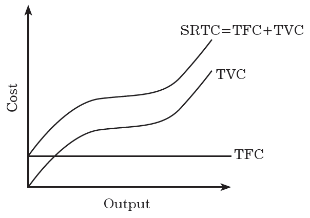
Short Run Total Costs Curves The total cost TC of business is the sum of the total variable costs TVC and total fixed costs TFC. From the diagram the following relationships can be discovered. In contrast, forty-eighth answered that they were constant, and simply forty-first answered that they had been attenuated. Stair-step Variable Costs These costs increase in a stair-step fashion as shown in Fig. Another characteristic of LRTC is that costs first increase at a decreasing rate until point B in Fig. Marginal cost defines the additional cost of producing each additional unit.
Reference: From the source of Wikipedia: Short-run marginal cost, Long-run marginal cost, Cost functions and relationship to average cost, From the source of Investopedia: What Is the Marginal Cost of Production, Example of Marginal Cost, From the source of Lumen Learning: Types of Costs, Total Cost, Variable Costs, Fixed Costs, Economic Cost,. To maximize efficiency, companies should strive to continue producing goods so long as marginal cost is less than marginal revenue. I am a Qualified Chartered Accountant, B. TFC remains constant even when the output is zero. Hence, the ATC curve falls as well. How to Calculate the Marginal Cost? The importance of marginal cost The marginal cost of production is used to optimize production levels.
Marginal Cost: Formula and Example Calculation Analysis
When used in conjunction with skilled planning and marketing, margin cost pricing Marginal revenue relative to a demand curve Usually, a firm would do this if they are suffering from weak demand, so reduce prices to marginal cost to attract customers back. Thus average variable cost has to fall. Answer: From the options given above, we can note that the costs of equipment, rent and interest payment on past borrowings are fixed in nature. It is usually calculated once enough things are created to hide the mounted prices and production is at a break-even purpose, wherever the sole expenses within the future area unit variable or direct prices. Finally, the known production function gives us the isoquant map, represented by Q 1, Q 2 and so forth.
However, without enough time to replace, upgrade, or sell fixed costs to react to an even larger volume, eventually the economies of scale reverse and the marginal cost goes up with increased production volume. This happens when the average cost curve reaches its lowest point. He manages to sell seventy thousand goods, making five lac pounds in revenue. Average fixed cost is relatively high at very low output levels. In combination with marginal cost analysis, businesses use variable and fixed costs for different types of financial analysis, trend monitoring, pricing, and decision-making. However, with gradual increase in output, AFC continues to fall as output increases, approaching zero as output becomes very large.
What Is Short Run Cost? Types: Total, Average, Marginal
This generates either the same profit level or a spike in profit if they raise prices higher than the inflation rate increases. You can see in Fig. Note that, while the AFC can become really small, it is never zero. The fixed factors of production are absent in the long run. In others, it refers to the speed of modification of total value as a little quantity will increase output. Economies of Scale : Various factors may give rise to economies of scale, that is, to decreasing long-run average costs of production.
Short Run Total Costs: Total Variable Costs and Total Fixed Costs
Column 4 shows the total cost of producing each level of output at the lowest possible cost. Once you have your total cost, you can figure out the average cost for each unit of the product or service you sell. At every production level and amount being thought of, incremental cost includes all prices fluctuating with the assembly level. Other costs do vary with the level of output produced by the firm during that time period. The total cost curve TC is obtained by adding the TFC and TVC vertically. By the end of July, you have sold 1300 total frames. It can be expressed as: So it is the ratio of MC to AC.
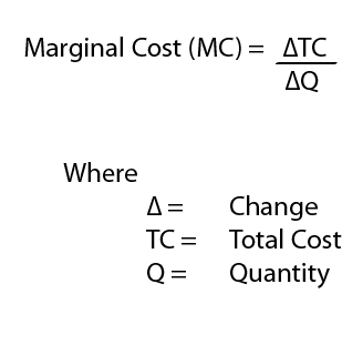
How to Calculate Marginal Cost Calculate marginal cost using the marginal cost formula, which measures the cost of producing one additional unit of goods or services provided to a customer. If a firm could sell the additional unit at a price greater than the cost incurred to produce the additional unit marginal cost , the firm may decide to produce the additional unit. As a result, although the short-term incremental cost rises owing to capacity constraints, the long-term incremental cost is often constant. These combinations enable us to locate seven points on the expansion path. But, on the other hand, several laborers could mean they spend more on wages than the output they are bringing in. When average cost decreases, marginal cost is less than average cost.
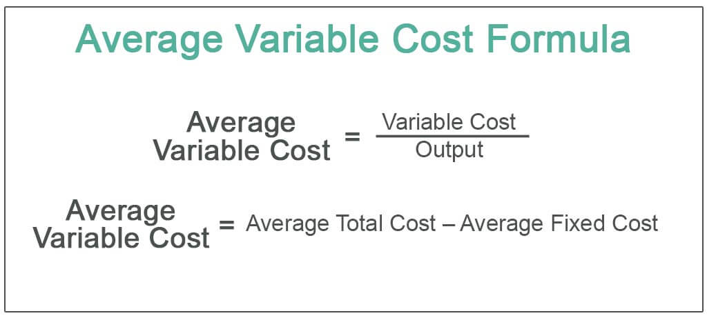
Average Variable Cost AVC The second aspect of short-run average costs is an average variable cost. Columns 6 and 7 depict that both average variable and average total cost first decrease, then increase, with average variable cost attaining a minimum at a lower output than that at which average total cost reaches its minimum. Long-run average cost first declines, reaches a minimum at Q 2 in Fig. The average cost curve falls till it reaches a certain point, and the marginal cost curve remains below that point. For instance, it may cost two hundred rupees to make five cups of Tea. First, costs and output are directly related; that is, the LRTC curve has a positive slope.