The long run average cost curve shows. When the long run average cost curve is downward sloping? 2022-12-08
The long run average cost curve shows Rating:
4,7/10
1684
reviews
The long run average cost curve is a graphical representation of the relationship between the long run average cost of producing a good or service and the level of output. It is an important concept in economics, as it helps firms understand how to minimize their costs and increase their profits in the long run.
In the long run, all factors of production are variable, meaning that firms have the ability to adjust the amount of inputs they use in the production process. This means that firms can choose the optimal combination of inputs to produce a given level of output, and the long run average cost curve reflects this optimization process.
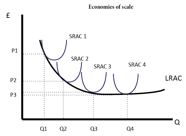
The long run average cost curve has several key features. First, it is typically U-shaped, with the minimum point of the curve representing the minimum efficient scale of production. This is the level of output at which the firm is able to achieve the lowest possible long run average cost. At this point, the firm is able to fully utilize its fixed inputs and achieve economies of scale, which are cost savings that result from increased production.
Beyond the minimum efficient scale, the long run average cost curve begins to rise. This is because as the firm increases its production, it may begin to face diminishing returns to its variable inputs, resulting in higher costs. Additionally, as the firm increases its production, it may also face increasing returns to scale, which can lead to lower costs.
The long run average cost curve is an important tool for firms to understand how to minimize their costs and increase their profits in the long run. By understanding the relationship between cost and output, firms can make informed decisions about their production levels and the optimal combination of inputs to use in the production process. This can help them remain competitive and successful in the long run.
Long Run Average Cost Curve: Derivation, Example, Solved Questions etc
Price-Volume Relationship Price-volume graphs are important for understanding how the firm's profit is related to how much they make. Economies and Diseconomies of Scale Notice that the long-run average cost curve in Why would a firm experience economies of scale? The future of cities, both in the United States and in other countries around the world, will be determined by their ability to benefit from the economies of agglomeration and to minimize or counterbalance the corresponding diseconomies. He concluded that companies should not use the largest machines available because of the outage danger and that they should not use the smallest size because that would mean forgoing the potential gains from economies of scale of larger sizes. In the United States, about 80% of the population now lives in metropolitan areas which include the suburbs around cities , compared to just 40% in 1900. The variable like increased output which leads to a higher average cost in an economy.
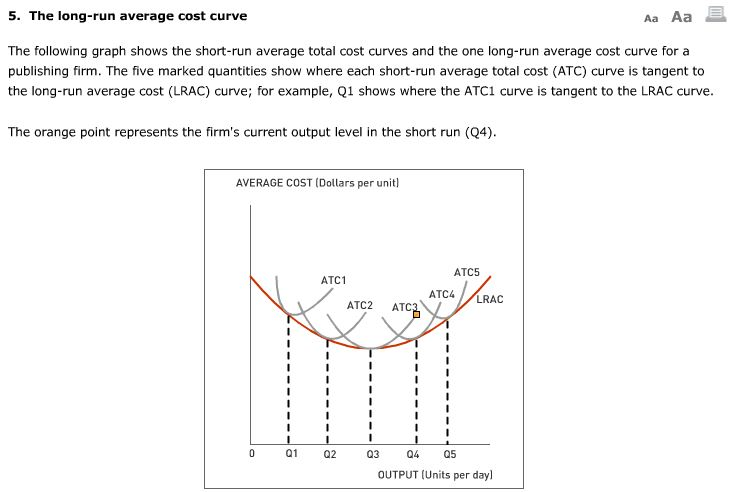
Answers to Try It! The implication here is that the beer industry is highly capital intensive. Different machine sizes are made with the same components and thus have essentially the same probability of breaking down. The following graph shows an example of a marginal cost curve for a firm in manufacturing. In its long-run planning, the firm not only regards all factors as variable, but it regards all costs as variable as well. Given that this long-run curve is drawn tangentially to all the increasingly graded SAC, it showcases the points with the lowest cost and thus gives the firm an idea of what SAC it can use to achieve the desired output. After closely examining each SAC also referred to as plants, there may be more than 3 for a single firm , the firm will need to determine the most optimal curve to maximize production and minimize cost. Economies of scale imply a downward-sloping long-run average cost LRAC curve.
In this case, a firm producing at a quantity of 10,000 will produce at a lower average cost than a firm producing, say, 5,000 or 20,000 units. Also, the corresponding SAC is SAC 2. On the other hand, to produce a higher output OV, the firm requires SAC 3. To enjoy these features, download the app or log in to the website now. In the graph on the right, the opposite is true.
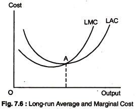
To find that point, we take the derivative of each curve and find where they are equal to one another. Summing up, we can say that in the long run, the firm employs the plant yielding maximum output at minimum cost per unit. It is based on the basic precept that the total cost of production is categorized into two. This example shows that as an input becomes more expensive in this case, the labor input , firms will attempt to conserve on using that input and will instead shift to other inputs that are relatively less expensive. This curve is used to determine the possible projections of cost and output for the long term. Then the price-quantity point is reached and quantity is increased.
As the curve slopes down the cost per unit shrinks as seen in the change from point A to point B. What shifts MC curve down? As the quantity of production rises, the variable costs also rise. The market demand in conjunction with the long-run average cost curve determines how many firms will exist in a given industry. In such a case, the smooth curve enveloping all these As you can see in the figure above, the long run average cost curve is drawn tangential to all SACs. The long-run cost curve is also referred to as the marginal cost of the plant.
Amazon Traditionally, bookstores have operated in retail locations with inventories held either on the shelves or in the back of the store. Many of the attractions of cities, like sports stadiums and museums, can operate only if they can draw on a large nearby population base. Visit this The Size and Number of Firms in an Industry The shape of the long-run average cost curve has implications for how many firms will compete in an industry, and whether the firms in an industry have many different sizes, or tend to be the same size. An additional unit of capital produces the marginal product of capital. This graph shows the cost of producing each unit of output. Solved Question on Long Run Average Cost Curve Q1.
When the LRAC curve has a flat bottom, then firms producing at any quantity along this flat bottom can compete. A long-run is different from a short-run in various factors and inputs. The costs it shows are therefore the lowest costs possible for each level of output. What is the shape of an average long run cost curve Why? At first, only a small amount of steel was produced. In the long run the firm can examine the average total cost curves associated with varying levels of capital. The second thing the firm can select is the scale or overall size of its operations. It will continue to transfer funds from capital to labor as long as it gains more output from the additional labor than it loses in output by reducing capital.
When the long run average cost curve is downward sloping?
The parts are molded in Texas border towns and are then shipped to maquiladoras and used in cars and computers. If firms in an industry experience economies of scale over a very wide range of output, firms that expand to take advantage of lower cost will force out smaller firms that have higher costs. The Factors Needed to Determine Short Run and Long-Run Cost Curves To determine the long-run total cost curve, an individual must know factors that affect changes in production. The graph to the right shows what happens when volume and price are both increased. The long-run average cost curve is used to plan the desired output for a specific cost, granting it the title of the planning curve. Here the point of the efficient scale is the LRAC curve with a minimum average cost for a firm. Such industries are likely to have a few large firms instead of many small ones.
The long run average total cost LRATC curve shows the A lowest average variable
The long-run average cost LRAC curve shows all possible output levels against an average cost In a U-shaped curve. This cost can be derived from short-run marginal cost. The LRAC curve assumes that the firm has chosen the optimal factor mix, as described in the previous section, for producing any level of output. For the range of output over which the firm experiences constant returns to scale, the long-run average cost curve is horizontal. Variable costs vary with the level of production. Then they remain constant for some time and eventually decrease. A firm can produce three different quantities of steel.
The law of diminishing marginal returns, after all, tells us how output changes as a single factor is increased, with all other factors of production held constant. However, high-efficiency turbines to produce electricity from burning natural gas can produce electricity at a competitive price while producing a smaller quantity of 100 megawatts or less. The long run cost curve helps us understand the functional relationship between out and the long run cost of production. Suppose Lifetime Disc Co. Its cost and demand information are given below. This shape depends on the returns to scale. It is more of a tool to determine which SAC would be ideal for a scenario.